Simulating New Data

Create a Simulation Object

Getting started with MASE is straightforward, let’s look at an example.

Covariance Matrix: Let’s simulate 5 indepedent features by setting this to the 5x5 identity matrix \(I\in \mathbb{R}^{5\text{x}5}\)

Means: Let’s choose each feature to have mean 0 by not supplying a means argument

N: Let’s generate 100 observations.

cov = np.eye(5)  # 5 independent features all with 0 mean
sim = Simulation(100, covariance_matrix=cov)  # 100 observations

Great! Now we have a Simulation object created and we can begin adding anomaly patterns.

Add Anomalies

First, let’s decide what anomalous behavior we would like to add to the data and store that information in a Pandas DataFrame called specs_df

specs_df = pd.DataFrame()
specs_df['mean'] = [3, 0]
specs_df['sd'] = [1, 2]
specs_df['n_obs'] = [20, 10]

specs_df now looks something like this:

mean	sd	n_obs
3 0	1 2	20 10

This dataframe corresponds to the adding of:

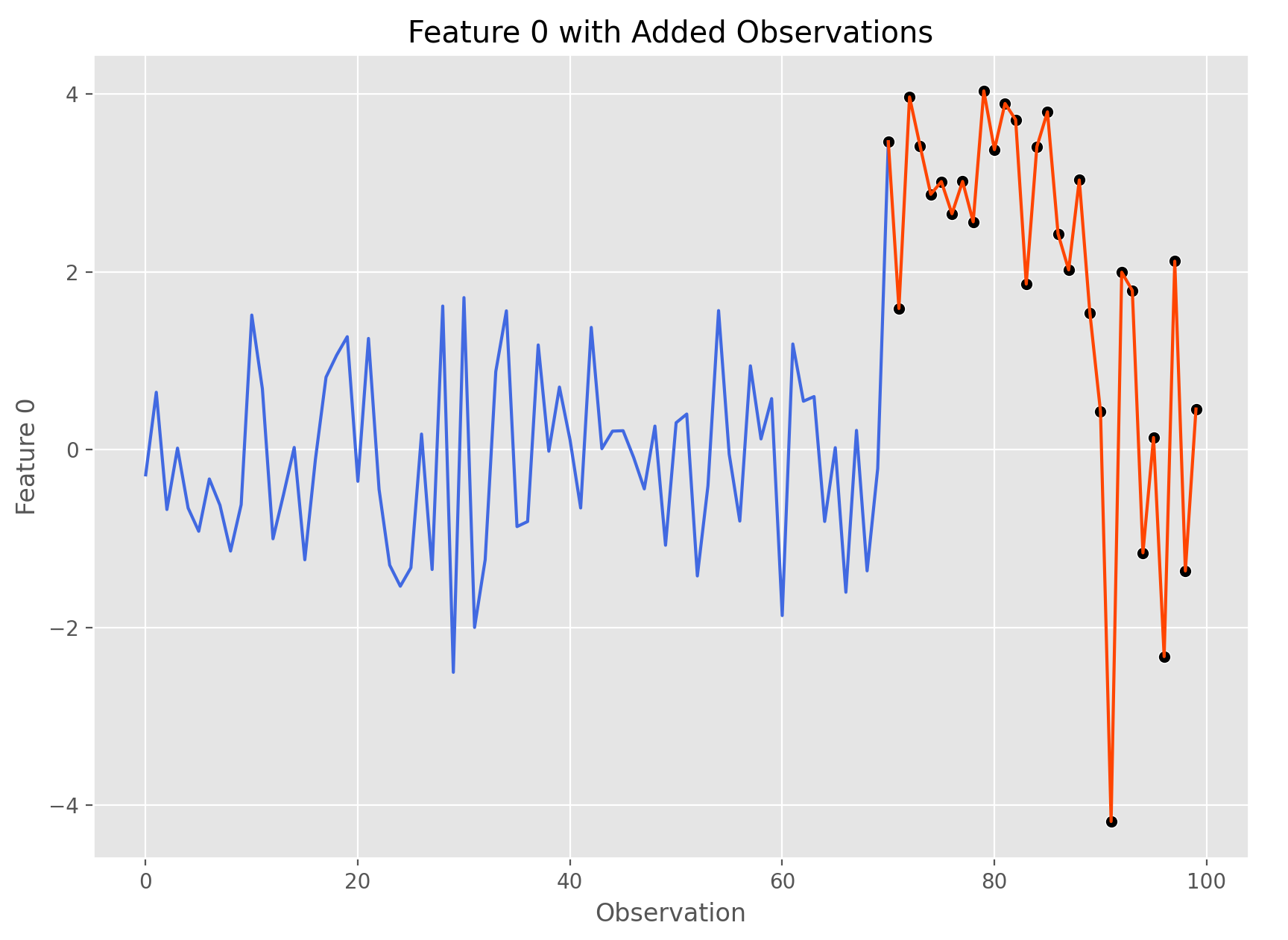
• 20 observations \(N \sim (3, \sigma)\)

• 10 observations \(N \sim (0, 2\sigma)\)

Let’s apply this to feature 0 in our data:

feature_index = 0
sim.add_gaussian_observations(specs_df, feature_index, visualize=True)

Go ahead and give this code a try yourself by running

mase.basic_demo()

Which runs the following function:

def basic_demo():
    cov = np.eye(5)  # 5 independent features all with 0 mean
    sim = Simulation(100, covariance_matrix=cov)  # 100 observations
    summary_df = pd.DataFrame()
    summary_df['mean'] = [3, 0]
    summary_df['sd'] = [1, 2]
    summary_df['n_obs'] = [20, 10]
    feature_index = 0
    d = sim.get_data()
    print(d)
    sim.add_gaussian_observations(summary_df, feature_index, visualize=True)